You need the following Simdify® modules to complete this exercise: Simdify® Free Edition, Simdify® Compute Module, Simdify® Buffer Module
This section describes common document layout and structures you'll encounter throughout these exercises. You can skip this section and move on to the exercises if you wish.
Through many of these exercises, we're going to follow a pattern where we use a compute shader to perform a particular workload, and then we'll use a vertex/fragment shader to visualize the results. Finally, we'll perform the compute dispatch and draw operations required to schedule work and get a result on-screen, or to read the work back from the GPU so it can be inspected and used in some way.
In general, we'll use more complicated compute shaders, we'll mutate an image or buffer variable, and then we'll visualize those results with a relatively simple vertex/fragment shader.
The order of nodes in the document, along with their grouping, has important features. In this view, you can see the document is broadly grouped into separate areas: Includes, Locals, Compute Shader, Horz Pass Resources, Vert Pass Resources, Visual Resources, Visual Shader, and Execute Workload. Note that you don't have to create these resources manually. In most cases, the software creates them for you.
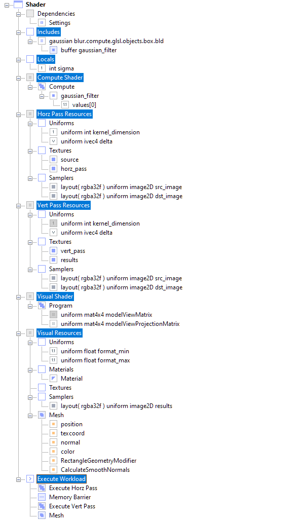
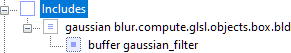
In the Includes section, <FileNode> and <NodeLink> objects store links to content in other documents. You can manually add content here as needed, and the software will also automatically add links here from time-to-time.
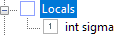
In the Locals section, you can declare <VariableNode> objects or other content that you need to make generally available in the document. In this example, we've declared an <Int32Node> named sigma that will be used to the strength of the Gaussian blur, but we don't need to use this value in the shader code itself. You can right click on Locals to create new <VariableNode> objects.
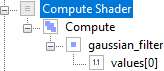
In the Compute Shader section, we connect the <Program> node to the compute shader source code on disk. Optionally, shader buffer and uniform buffer resources are defined and bound here.
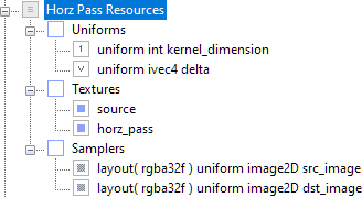
In the Horz Pass Resources section we define uniform, texture, and sampler resources for the horizontal compute pass.
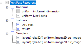
In the Vert Pass Resources section we define uniform, texture, and sampler resources for the vertical compute pass. Note that we disable one of the uniforms already specified by the horizontal pass since we don't want to set its value twice. However, we could set different uniform values here if needed.
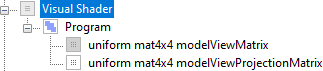
In the Visual Shader section, we connect the <Program> node to the vertex/fragment shader source on disk. Sometimes you won't be using a compute shader for workloads that generate final results, but we'll still use this section since it's useful to be able to get data from the compute shader for debugging purposes.
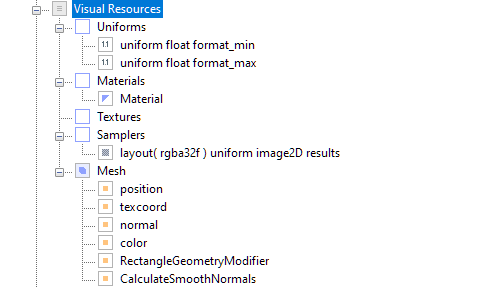
In the Visual Resources section, we specify uniforms, textures, samplers, materials, and a mesh used to render results if desired.
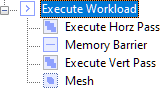
In the Execute Workload section, we schedule work via node rendering order. The first test occurs with the <GraphicsFeatureNode> named Execute Workload, which performs tests against the graphics hardware to determine whether or not to perform any of the specified workload based on the GLSL version and any required extensions. For example, this workload will not execute on a machine without a GLSL compiler of version 400 or higher. Execute Workload displays a red underline if it fails, and you can move the mouse over the node to learn about the error.
Once the application determines that it can perform the workload, it traverses Execute Horz Pass first, which executes the compute shader workload and then returns. Next, the application encounters a memory barrier, which means that it waits until the GPU workload is complete before proceeding. Then it traverses Execute Vert Pass, which executes the compute shader workload again with different uniform values for delta.
Finally, it traverses Mesh, which starts the chain reaction that renders the image sampler mutated by the compute shader onto the mesh geometry. It's important to understand that the <Mesh> is just a link to the actual mesh. This link technology allows you to configure documents without resorting to copy and paste.